Race Conditions Can Be Useful for Parallelism
Many are well aware of the hazards of race conditions. But what about the benefits?
There are situations where race conditions can be helpful for performance. By this, I mean that you can sometimes make a program faster by creating race conditions. Essentially, a small amount of non-determinism can help eliminate a performance bottleneck.
Now, first, let me emphasize: I’m not talking about data races. Data races are typically bugs, by definition.1 Instead, I’m talking about how to utilize atomic in-place updates and accesses (e.g., compare-and-swap, fetch-and-add, etc.) to trade a small amount of non-determinism for improved performance.
Two interesting examples are priority updates and deterministic reservations. Both techniques are able to ensure some degree of determinism, and yet are non-deterministic “under the hood”. In this post, we’ll look at priority updates.
It’s important for parallel programmers to be aware of these techniques for a couple reasons. First, the performance advantages (for both space and time) are significant. But perhaps more importantly, these techniques demonstrate that race conditions can be disciplined, possible to reason about, and useful.
Example: Parallel Breadth-First Search (BFS)
It’s helpful to have a motivating example, so let’s consider a parallel breadth-first search. This algorithm operates in a series of rounds, where on each round it visits a frontier of vertices which are all the same distance from the source (the initial vertex). By selecting the subset of edges which are “used” to traverse the graph, we derive a BFS tree. In the BFS tree, each vertex points to its parent, which is a vertex from the previous frontier.
For example, below is a graph with vertices labeled 0 through 9. The second image shows one possible BFS tree, with frontiers highlighted, starting with vertex 0 as the source. In this graph, the maximum distance from the source is 3, so there are 4 frontiers (corresponding to distances 0, 1, 2, and 3).
 input graph input graph |
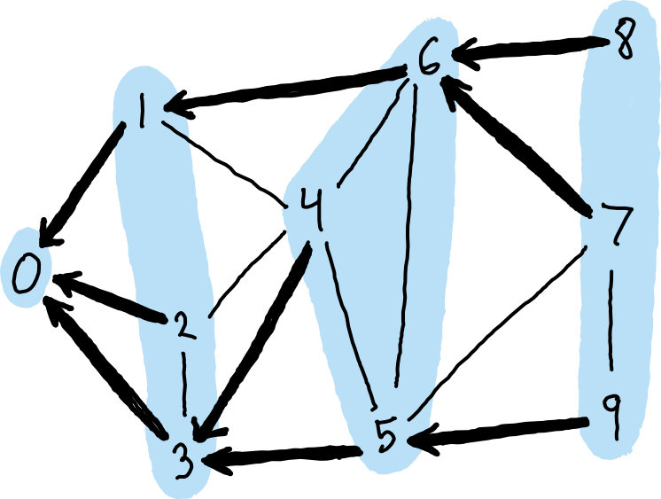 BFS tree (bold edges) and frontiers (highlighted) BFS tree (bold edges) and frontiers (highlighted) |
Selecting Parents in Parallel
On each round of BFS, we have a frontier of vertices, and we need to compute the next frontier. To do so, we need to select a parent for each vertex.
Selecting a parent for each vertex requires care, because for each vertex, there might be multiple possible parents. For example, in the images above, vertex 3 was selected as the parent of vertex 4, but either vertex 1 and 2 could have been selected instead.
How should we go about selecting parents? Below, we’ll consider three options: one which is race-free, one which has race conditions but is significantly faster, and one which has race conditions but is able to ensure deterministic output.
Slow approach: collect potential parents and then deduplicate
The idea here is to first compute the set of potential parents, and then select parents from these. The potential parents are a list of pairs \((v,u)\) where \(u\) could be selected as the parent of \(v\). From these, we can select parents by “deduplicating”: for any two pairs \((v, u_1)\) and \((v, u_2)\), we keep one and remove the other (and continue until there are no duplicates).
One nice thing about this approach is that it is easy to make deterministic. Deduplication can (for example) be implemented by first semisorting to put duplicate pairs in the same bucket, and then by selecting one element from each bucket. This results in deterministic parent selection in linear work and polylog depth.
However, one not-so-nice thing about this approach is that it is slow, because it stores the set of potential parents in memory. Across the whole BFS, every edge will be considered as a potential parent once. Therefore, constructing the set of potential parents incurs a total of approximately \(2|E|\) writes to memory for \(|E|\) edges in the input graph. (The factor of 2 is due to representing potential parents as a list of pairs.)
That’s a lot of memory traffic which could be avoided.
Faster approach: deduplicate “on-the-fly”
To speed things up, we can do deduplication more eagerly while generating the set of potential parents. The result is that the set of potential parents never needs to be fully stored in memory.
We’ll operate on a mutable array, where each cell
of the array stores the parent of a vertex. Initially, these are all “empty”
(using some default value, e.g., -1). To visit a vertex, we set its parent
by performing a compare-and-swap,
or CAS for short.
In particular, suppose that vertex \(u\) is a potential parent of \(v\). The
following ML-like pseudocode implements a function
tryVisit(v,u) which attempts to set \(u\) as the parent of \(v\), and returns
true if successful, or false if \(v\) has already been visited. The code
is implemented in terms of a function compareAndSwap(a, i, x, y) which
performs a CAS at a[i], returning a boolean of whether or not
it successfully swapped from x to y.
(* Mutable array of parents. `parents[v]` is the parent of `v`,
 * or `-1` if `v` has not yet been visited. *)
val parents: vertex array = ...

(* Try to set `u` as the parent of `v`.
 * Returns a boolean indicating success. *)
fun tryVisit(v,u) =
  parents[v] == -1 andalso compareAndSwap(parents, v, -1, u)
On one round of BFS, we can then apply tryVisit(v,u) in parallel for every
newly visited vertex \(v\) and each of its potential parents \(u\). This
requires traversing the set of potential parents, but does not require storing
it in memory.
This performs one compare-and-swap per edge. Assuming relatively low contention, this requires only approximately \(|V|\) memory updates in total (where \(|V|\) is the number of vertices) across the whole BFS: for each vertex, there will be one successful CAS. That is a significant improvement over the \(2|E|\) updates required for the slower approach.
Non-determinism. This approach ensures that some parent is selected for each vertex, but doesn’t ensure that the same parent will be selected every time. Therefore, the final output of the BFS, while always correct, could be different on each execution. (There are many valid BFS trees for any graph, and the above algorithm selects one of them non-deterministically.)
Regardless of non-determinism, we can still argue that this code is correct.
There is a race condition to reason about: any two
calls tryVisit(v,u1) and tryVisit(v,u2)
will race to update the value parents[v].
Abstractly, each value parents[v] has only two possible states: either
“empty” (i.e., -1), or set with a valid parent. If a CAS
succeeds, then the resulting value parents[v] is valid and will never change.
If a CAS fails, then another CAS on the same cell must have succeeded.
Making it deterministic with priority updates
To make the above approach deterministic, we can use priority updates. The idea is to select the “best” parent on-the-fly using CAS. We’ll say that a parent \(u_1\) is “better than” some other parent \(u_2\) if \(u_1 > u_2\) (relying on numeric labels for vertices). So, in other words, we want to compute the maximum parent for each vertex.
Here’s some pseudocode. Again, we use a mutable array
parents where parents[v] is the parent of v, or -1 if it has not
yet been visited. We additionally need a second mutable array, visited,
where visited[v] is a boolean indicating whether or not a vertex has
been visited yet. This ensure that we only update the parents of unvisited
vertices. At the end of each round, the visited flags for the new frontier
need to be updated.
val parents: vertex array = ... (* same as before *)
val visited: bool array = ... (* visited flags for each vertex *)

(* Try to make `u` the parent of `v`, but only if
 *   1. `v` has not yet been visited, and
 *   2. `u` is a "better" parent (i.e., larger)
 * Returns a boolean indicating whether or not the
 * first update was performed. *)
fun priorityUpdateParent(v,u) =
  if visited[v] then
    false
  else
  let
    val old = parents[v]
    val isFirstVisit = old == -1
  in
    if u <= old then
      false  (* done: better parent already found *)
    else if compareAndSwap(parents, v, old, u) then
      isFirstVisit  (* done: successful update! *)
    else
      priorityUpdateParent(v,u)  (* retry: CAS contention *)
  end
We apply priorityUpdateParent(v,u) in parallel for every
to-be-visited vertex \(v\) and each of its potential parents \(u\). This
requires traversing all potential parents, but does not require storing
them in memory. (For more details, see the full code below.)
When this completes, the “best” parent (i.e., the one with
largest numeric label) will have been selected for each vertex.
Therefore, the output is deterministic.
Note that, although this produces deterministic output, the algorithm itself
is non-deterministic. There is a race condition to reason about: any two
contending calls priorityUpdateParent(v,u1) and priorityUpdateParent(v,u2)
will race to update the value parents[v].
To argue correctness, consider that each value parents[v]
increases monotonically with each successful CAS. With this observation,
it’s not too difficult to brute force through all
possible interleavings of loads and CAS operations to see that the code is
correct. Essentially, each call to priorityUpdateParent has a
linearization point
at the moment it performs a successful CAS. At this linearization point,
the state of the cell increases monotonically. After all calls complete, the
final value of the cell is the maximum.
If you are unfamiliar with this kind of reasoning, I would highly encourage spending an hour or two working through it!
Cost. How many memory updates does this approach require? That is a really interesting question, and the answer is not so straightforward. In their paper, Shun et al. consider multiple reasonable models and argue that for \(n\) contending priority updates, we can expect approximately \(O(\log n)\) successful CAS operations. In the context of BFS, the variable \(n\) corresponds to the maximum degree of a vertex, as this will be the maximum number of contending priority updates. Therefore, the total number of memory updates in this approach will be approximately \(|V| \log \delta\), where \(\delta\) is the maximum degree of any vertex. Not bad!
Implementation of Deterministic BFS with Priority Updates
Below is the code for a deterministic parallel breadth-first search using
priority updates to select parents. It’s written in a mostly functional style,
using standard
data-parallel functions like map, filter, flatten, etc., as well
compare-and-swap operations to implement the priority update. This code
is similar to Parallel ML, which we could compile and run with
the mpl compiler.
The function breadthFirstSearch(G,s) performs a
breadth-first search of graph G, starting from a vertex s.
We assume vertices are integers, labeled 0 to N-1. The search returns an
array of parents, with one parent for each vertex. In the array of parents, a
value of -1 is used to mark unvisited vertices (i.e., vertices without a
parent). This way, the array of parents serves two purposes: it will be the
output, but also, it is used to indicate which vertices have been visited.
BFS begins by allocating the array of parents, initializing with -1 for
each vertex, indicating that no vertices have been visited yet. The BFS then
proceeds in a series of rounds, where each round takes as argument the
frontier of the previous round. We then compute the next frontier by
selecting parents as described above.
The BFS terminates as soon as the current frontier is empty, which occurs as soon as all vertices reachable from the source have been visited.
fun breadthFirstSearch(G: graph, source: vertex) : vertex array =
  let
    val parents: vertex array = tabulate(numVertices(G), fn v => -1)
    val visited: bool array = tabulate(numVertices(G), fn v => false)

    (* Try to update parent[v] := u, but only if v has not yet been
     * visited, and if u is larger than the previous parent. After
     * all priority updates have completed, the parent of v
     * will be the maximum of all potential parents.
     * Returns a boolean indicating whether or not the first update
     * of parent[v] was performed. This is used by the filter below
     * (see tryUpdateParents) to deduplicate.
     *)
    fun priorityUpdateParent(v,u) =
      if visited[v] then
        false
      else
      let
        val old = parents[v]
        val isFirstVisit = old == -1
      in
        if u <= old then
          false  (* done: better parent already found *)
        else if compareAndSwap(parents, v, old, u) then
          isFirstVisit  (* done: successful update! *)
        else
          priorityUpdateParent(v,u)  (* retry: CAS contention *)
      end

    fun tryUpdateParents(u) =
      filter(neighbors(G,u), fn v => priorityUpdateParent(v,u))

    (* One round of BFS. The frontier is the set of vertices
     * visited on the previous round. *)
    fun computeNextFrontier(frontier: vertex array) : vertex array =
      let
        val nextFrontier = flatten(map(frontier, tryUpdateParents))
      in
        (* visit the next frontier *)
        foreach(nextFrontier, fn v => visited[v] := true);
        nextFrontier
      end

    fun bfsLoop(frontier: vertex array) =
      if size(frontier) = 0 then () (* done *)
      else bfsLoop(computeNextFrontier(frontier))

    val firstFrontier = singletonArray(s)
  in
    parents[s] := s;        (* visit source (use self as parent) *)
    visited[s] := true;
    bfsLoop(firstFrontier); (* do the search *)
    parents                 (* return array of parents *)
  end
Some Timings
Below are timings collected from the Parallel ML Benchmark Suite for the three BFS strategies discussed here. These three strategies vary in their level of determinism: one is fully deterministic, one is partially deterministic (i.e. deterministic output but not non-deterministic execution), and one is completely non-deterministic.
The table shows timings on \(P = 1\) and \(P = 72\) processors, and speedups relative to a baseline 1-processor time. The speedup is computed as \(T_{72} / B\), where \(T_{72}\) is the time on 72 processors and \(B\) is the baseline; in this case, we use the fastest 1-processor time as the baseline. The input is a randomly generated power-law graph, with approximately 16.8M vertices and 199M edges, symmetrized.
We can see here that the fastest approach is the fully non-deterministic strategy. Not far behind (~20% slower) is the approach based on deterministic priority updates. And, by far, the slowest approach is the fully deterministic strategy. The additional cost for the fully deterministic strategy is due to high memory pressure, to write out all potential parents before duplicating.
| BFS Strategy | Deterministic? | P = 1 | P = 72 | Speedup (w.r.t. fastest 1-proc) |
|---|---|---|---|---|
| race-free, explicit dedup (slow approach) | yes | 89.6s | 1.84s | 8x |
| deterministic priority updates | output only | 18.7s | 0.487s | 30x |
| deduplicate on-the-fly (faster approach) | no | 14.8s | 0.406s | 36x |
Final Thoughts
In cases where non-determinism is acceptable, the results above demonstrate that race conditions can be useful for improving performance. But this improved performance comes with the tradeoff: racy code is more difficult to debug and prove correct.
In my experience, with a bit of practice, reasoning about race conditions can become familiar and comfortable. It’s especially helpful to acquire a repertoire of familiar techniques. Knowing just a few techniques is sufficient for understanding a wide variety of sophisticated, state-of-the-art parallel algorithms. Priority updates are a great place to get started.
If you’re interested in learning more, consider reading about deterministic reservations, a technique for parallelizing incremental sequential algorithms. The resulting algorithms are parallel, with deterministic output, but non-deterministic execution. The technique is surprisingly powerful.
Footnotes
-
In the context of a language memory model, a data race is typically defined as two conflicting concurrent accesses which are not “properly synchronized” (e.g., non-atomic loads and stores, which the language semantics may allow to be reordered, optimized away, etc). Data races can lead to incorrect behavior due to miscompilation or lack of atomicity, and are therefore often considered undefined behavior. In other words, in many languages (e.g. C/C++), data races are essentially bugs by definition. One recent exception is the OCaml memory model, which is capable of providing a reasonable semantics to programs with data races. See Bounding Data Races in Space and Time, by Stephen Dolan, KC Sivaramakrishnan, and Anil Madhavapeddy. ↩
Comments
Cool article
Thanks Bob!